The Four Fundamental Subspaces

• The Problem of Solving Linear Equations
• Basis, Dimension, and Rank
  • Basis
  • Dimension
  • Rank
  • Dimension vs Rank
• The Four Fundamental Subspaces
  • The Column Space C(A)
  • The Nullspace N(A)
  • The Row Space C(A^T)
  • The Left Nullspace N(A^T)
• Integrating Concepts: The Complete Solution
  • How many solutions are there?
• Summary: The Fundamental Theorem of Linear Algebra
  • The Fundamental Theorem
• Guided Problems
  • Problem 1: Rank-One Matrices and the Four Fundamental Subspaces
  • Problem 2: Nullspace Preservation and the Gram Matrix
• References

---

The Problem of Solving Linear Equations

We want to solve a system of $m$ linear equations in $n$ unknowns, written as $Ax=b$. In the "row picture," each of these $m$ equations defines a hyperplane in $n$-dimensional space. The goal is to find a solution $x$, which is a single point of intersection that lies on all $m$ of these hyperplanes.

This geometric view presents three possibilities:

1. One Solution: The hyperplanes intersect at a single point.
2. No Solution: The hyperplanes have no common intersection point (e.g., two planes are parallel).
3. Infinite Solutions: The hyperplanes intersect on a larger set, such as a line or a plane (e.g., three planes intersect on a common line).

The homogeneous case $Ax=0$ is a related problem where $b=0$. Since all hyperplanes must pass through the origin, $x=0$ (the "trivial solution") is always one answer. The fundamental question becomes: Do the hyperplanes intersect only at the origin, or do they also intersect along a larger set (like a line or plane) that passes through the origin?

---

Basis, Dimension, and Rank

Basis

You can represent every vector in $R^2$ with combinations of the two vectors $\left\{ \begin{bmatrix} 1 \\ 0 \end{bmatrix}, \begin{bmatrix} 0 \\ 1 \end{bmatrix} \right\}$ (orthonormal basis). It's also possible with $\left\{ \begin{bmatrix} 1 \\ 1 \end{bmatrix}, \begin{bmatrix} 1 \\ -1 \end{bmatrix} \right\}$ (orthogonal basis) or even $\left\{ \begin{bmatrix} 1 \\ 0 \end{bmatrix}, \begin{bmatrix} 1 \\ 1 \end{bmatrix} \right\}$ (non-orthogonal basis).

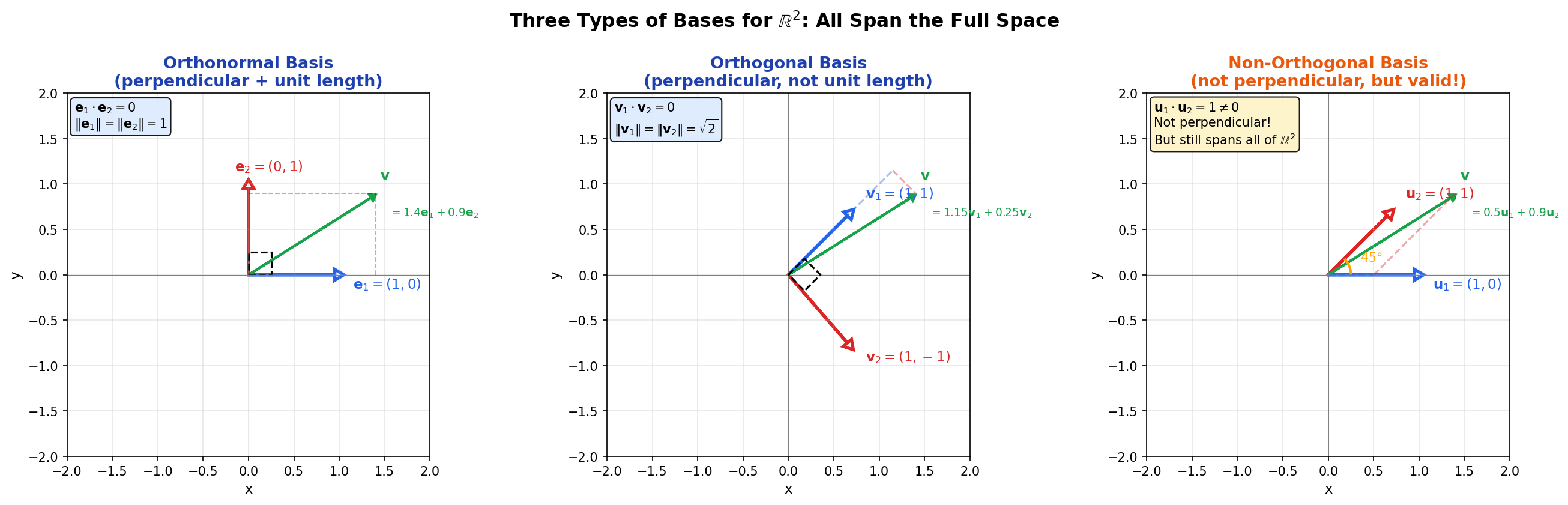
Figure: Three types of bases for $\mathbb{R}^2$. Left: Orthonormal basis. Middle: Orthogonal basis. Right: Non-orthogonal basis (not perpendicular, but still linearly independent and spans all of $\mathbb{R}^2$).

The same vector $\mathbf{v}$ (shown in green) has different coordinate representations in each basis.

• In the orthonormal basis (perpendicular and unit length), $\mathbf{v} = 1.4\mathbf{e}_1 + 0.9\mathbf{e}_2$.
• In the orthogonal basis (perpendicular but not unit length), $\mathbf{v} = 1.15\mathbf{v}_1 + 0.25\mathbf{v}_2$.
• In the non-orthogonal basis, $\mathbf{v} = 0.5\mathbf{u}_1 + 0.9\mathbf{u}_2$.

The dashed lines show how $\mathbf{v}$ is decomposed along each basis. Despite the different coefficients, all three representations describe the exact same point $(1.4, 0.9)$ in $\mathbb{R}^2$.

However, you cannot represent every vector in $\mathbb{R}^2$ with combinations of two linearly dependent vectors like $\left\{ \begin{bmatrix} 1 \\ 1 \end{bmatrix}, \begin{bmatrix} 2 \\ 2 \end{bmatrix} \right\}$. Since the second vector is just $2$ times the first, they point in the same direction and only span a one-dimensional line (the blue shaded region in the diagram below), not the entire two-dimensional plane.

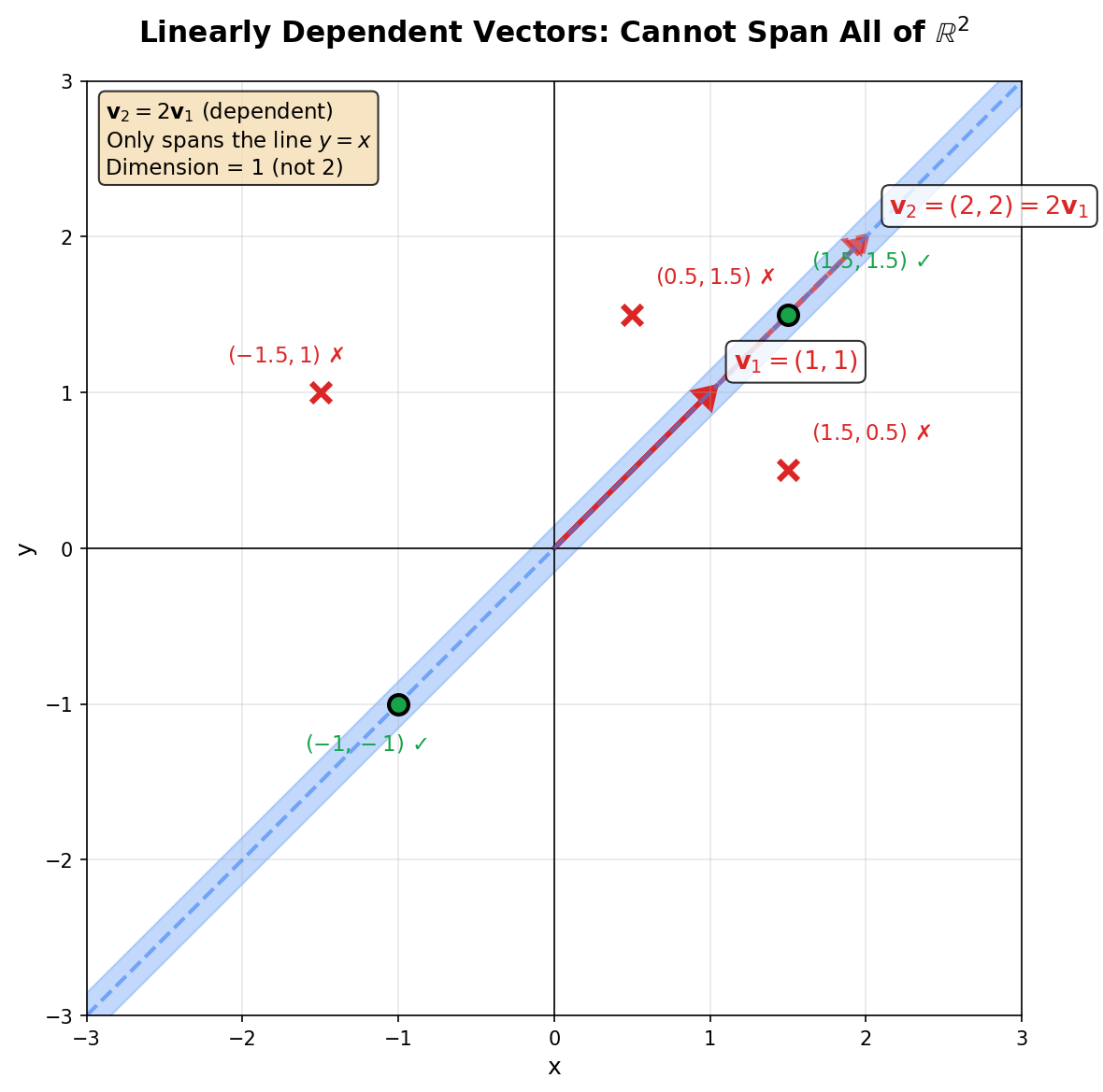
Figure: Linearly dependent vectors cannot span all of $\mathbb{R}^2$. Vectors on the line $y = x$ (green ✓) can be represented, but vectors off the line (red ✗) cannot.

From these examples, we observe a fundamental pattern: any set of linearly independent vectors can span a vector space and serve as a coordinate system to represent every vector in that space. In contrast, linearly dependent vectors (or a single vector alone) cannot span the entire space. This observation leads us to the formal definition of a basis—the minimal set of "building blocks" or "coordinate axes" for a vector space. A basis has just enough vectors: not too few (or it couldn't span the whole space) and not too many (or the vectors would be dependent, making some redundant).

Definition: Basis

A basis for a vector space $V$ is a set of vectors $\{v_1, \dots, v_k\}$ that satisfies both of the following properties:

1. Linearly Independent: The only solution to $c_1v_1 + \dots + c_kv_k = 0$ is when all coefficients $c_i = 0$. This means there is no redundancy—no vector in the set can be written as a combination of the others.

2. Spans the Space: Every vector $v \in V$ can be expressed as a linear combination $v = c_1v_1 + \dots + c_kv_k$ for some scalars $c_1, \dots, c_k$.

Dimension

From the examples above, we see that any vector in $\mathbb{R}^2$ can be represented by a linear combination of exactly two basis vectors, while any vector in $\mathbb{R}^3$ requires exactly three basis vectors. This number of vectors in a basis is the dimension of the space—it measures the "degrees of freedom" or the number of independent directions in that space. All bases for the same vector space contain the same number of vectors.

Theorem: The Basis Theorem

Let $V$ be a vector space with a finite basis. Then every basis for $V$ contains exactly the same number of vectors.

Definition: Dimension

The dimension of a vector space $V$, denoted $\dim(V)$, is the number of vectors in any basis for $V$.

Examples:

• A line has dimension 1.
• A plane has dimension 2.
• $\mathbb{R}^n$ has dimension $n$.
• If the nullspace of $A = \begin{bmatrix} 1 & 1 \\ 2 & 2 \end{bmatrix}$ is the line spanned by $\begin{bmatrix} 1 \\ -1 \end{bmatrix}$, then $\dim(N(A)) = 1$.

Rank

Consider the matrix $A = \begin{bmatrix} 1 & 2 \\ 2 & 4 \end{bmatrix}$. The second column is twice the first column, making them linearly dependent. Both columns lie on the same line in $\mathbb{R}^2$. All vectors that can be created by combining these columns span only a one-dimensional line, not the full two-dimensional plane. The number of linearly independent columns (or equivalently, the dimension of the space they span) is 1. This number is called the rank of the matrix.

The rank measures how many independent columns a matrix has. This always equals the number of independent rows.

Definition: Rank

The rank of a matrix $A$, denoted $\text{rank}(A)$ or $r$, is the dimension of its column space: $\text{rank}(A) = \dim(C(A))$.

Theorem: The Rank Theorem

The dimension of the column space equals the dimension of the row space. $\dim(C(A)) = \dim(C(A^T)) = r$ Consequently, the number of pivot positions in $A$ is equal to the rank of $A$.

How to Find Rank: The rank $r$ equals the number of pivots found by Gaussian elimination in the echelon form $U$ or reduced row echelon form $R$.

Example: $A = \begin{bmatrix} 1 & 2 & 3 \\ 2 & 4 & 6 \end{bmatrix} \xrightarrow{\text{elimination}} U = \begin{bmatrix} 1 & 2 & 3 \\ 0 & 0 & 0 \end{bmatrix}$

This matrix has only one pivot (the 1 in position (1,1)), so $\text{rank}(A) = 1$.

Dimension vs Rank

Dimension and rank are related but describe different objects:

Feature	Dimension	Rank
What it describes	A vector space or subspace	A matrix
What it measures	The number of vectors in any basis for the space	The number of independent columns (or rows) in the matrix
How to find it	Find a basis for the space and count the vectors	Count the pivots in the echelon form
Example	$\mathbb{R}^3$ has dimension 3 A plane in $\mathbb{R}^3$ has dimension 2 A line has dimension 1	A $3 \times 5$ matrix with 2 pivots has rank 2 A $100 \times 100$ matrix where all columns are multiples of one vector has rank 1

---

The Four Fundamental Subspaces

To answer the questions we stated at first, let's consider the $m \times n$ matrix $A$ below. For our examples, we will use this $3 \times 3$ matrix $A$ with rank $r=2$:

$A = \begin{bmatrix} 1 & 1 & 2 \\ 2 & 3 & 5 \\ 3 & 4 & 7 \end{bmatrix} \xrightarrow{\text{Elimination}} U = \begin{bmatrix} 1 & 1 & 2 \\ 0 & 1 & 1 \\ 0 & 0 & 0 \end{bmatrix} \xrightarrow{\text{Reduced Form}} R = \begin{bmatrix} 1 & 0 & 1 \\ 0 & 1 & 1 \\ 0 & 0 & 0 \end{bmatrix}$

The Column Space $C(A)$

Consider the columns of our matrix $A$: $c_1 = \begin{bmatrix} 1 \\ 2 \\ 3 \end{bmatrix}$, $c_2 = \begin{bmatrix} 1 \\ 3 \\ 4 \end{bmatrix}$, and $c_3 = \begin{bmatrix} 2 \\ 5 \\ 7 \end{bmatrix}$. Notice that $c_1 + c_2 = c_3$, so the third column is linearly dependent on the first two. All linear combinations of these three columns produce the same set of vectors as combinations of just $c_1$ and $c_2$. This set forms a 2-dimensional plane in $\mathbb{R}^3$, not the full 3-dimensional space.

This set of all linear combinations of the columns is called the column space $C(A)$. It answers a fundamental question: which vectors $b$ can we reach by solving $Ax = b$? When we write $Ax = b$ with $x = \begin{bmatrix} x_1 \\ x_2 \\ x_3 \end{bmatrix}$, we are asking whether we can find coefficients $x_1, x_2, x_3$ such that $x_1 c_1 + x_2 c_2 + x_3 c_3 = b$. This is precisely asking whether $b$ can be written as a linear combination of the columns. Therefore, $Ax = b$ has a solution if and only if $b \in C(A)$.

Definition: Column Space

The column space $C(A)$ of an $m \times n$ matrix $A$ is the set of all linear combinations of the columns of $A$. Equivalently, $C(A) = \{Ax : x \in \mathbb{R}^n\}$.

It is a subspace of $\mathbb{R}^m$.

Key Properties:

Property	Description	Our Example
Solvability	$b \in C(A) \iff Ax = b$ has a solution	$b$ must be in the plane spanned by columns 1 and 2
Dimension	$\dim(C(A)) = \text{rank}(A) = r$	$\dim(C(A)) = 2$
Basis	The $r$ pivot columns from $A$	$\left\{ \begin{bmatrix} 1 \\ 2 \\ 3 \end{bmatrix}, \begin{bmatrix} 1 \\ 3 \\ 4 \end{bmatrix} \right\}$

Finding the Basis: Identifying Pivot Columns

To find a basis for $C(A)$, perform Gaussian elimination to identify the pivot columns:

$A = \begin{bmatrix} 1 & 1 & 2 \\ 2 & 3 & 5 \\ 3 & 4 & 7 \end{bmatrix} \xrightarrow{\text{elimination}} U = \begin{bmatrix} \boxed{1} & 1 & 2 \\ 0 & \boxed{1} & 1 \\ 0 & 0 & 0 \end{bmatrix}$

The pivots (boxed) are in columns 1 and 2. The basis for $C(A)$ consists of the corresponding columns from the original matrix $A$ (not from $U$):

$C(A) = \text{span}\left\{ \begin{bmatrix} 1 \\ 2 \\ 3 \end{bmatrix}, \begin{bmatrix} 1 \\ 3 \\ 4 \end{bmatrix} \right\}$

Important: Always use the original columns, not the columns from the echelon form. Elimination changes the column space but preserves which columns are independent.

The Nullspace $N(A)$

Recall that our matrix $A$ has the dependency $c_1 + c_2 = c_3$. We can rewrite this as $c_1 + c_2 - c_3 = 0$, or equivalently: $A \begin{bmatrix} 1 \\ 1 \\ -1 \end{bmatrix} = 1 \cdot c_1 + 1 \cdot c_2 + (-1) \cdot c_3 = \begin{bmatrix} 0 \\ 0 \\ 0 \end{bmatrix}$

The vector $\begin{bmatrix} 1 \\ 1 \\ -1 \end{bmatrix}$ is a "recipe" that combines the columns to produce zero. This recipe encodes the dependency relationship among the columns. The set of all such recipes is called the nullspace $N(A)$.

In contrast, consider the identity matrix $B = \begin{bmatrix} 1 & 0 \\ 0 & 1 \end{bmatrix}$ with linearly independent columns. To find vectors $x$ such that $Bx = 0$: $x_1 \begin{bmatrix} 1 \\ 0 \end{bmatrix} + x_2 \begin{bmatrix} 0 \\ 1 \end{bmatrix} = \begin{bmatrix} 0 \\ 0 \end{bmatrix}$ The only solution is $x_1 = 0$ and $x_2 = 0$, giving $x = \begin{bmatrix} 0 \\ 0 \end{bmatrix}$. The nullspace contains only the zero vector, $N(B) = \{0\}$, confirming the columns are independent.

The nullspace reveals the redundancy in a matrix. If $N(A) = \{0\}$ (only the zero vector), the columns are independent. If $N(A)$ contains non-zero vectors, the columns are dependent. The nullspace also determines solution uniqueness: if $x_p$ solves $Ax = b$, then the complete solution set is $x_p + x_n$ for all $x_n \in N(A)$.

Definition: Nullspace

The nullspace $N(A)$ of an $m \times n$ matrix $A$ is the set of all solutions to the homogeneous equation $Ax = 0$. That is, $N(A) = \{x \in \mathbb{R}^n : Ax = 0\}$.

It is a subspace of $\mathbb{R}^n$.

Theorem: Rank-Nullity Theorem

The rank of a matrix $A$ plus the dimension of its nullspace equals the number of columns of $A$: $\text{rank}(A) + \dim(N(A)) = n$

Key Properties:

Property	Description	Our Example
Dimension	$\dim(N(A)) = n - r$ (number of free variables)	$\dim(N(A)) = 3 - 2 = 1$
Basis	Special solutions (set each free variable to 1)	$\left\{\begin{bmatrix} -1 \\ -1 \\ 1 \end{bmatrix}\right\}$ (a line in $\mathbb{R}^3$)
How to find	From $R = \begin{bmatrix} 1 & 0 & 1 \\ 0 & 1 & 1 \\ 0 & 0 & 0 \end{bmatrix}$: set $x_3 = 1 \implies x_1 = -1, x_2 = -1$	$x_1 + x_3 = 0$ and $x_2 + x_3 = 0$

Finding the Basis: Solving $Ax = 0$ from Reduced Form

To find a basis for $N(A)$, reduce the matrix to reduced row echelon form (RREF) and solve $Rx = 0$:

$R = \begin{bmatrix} 1 & 0 & 1 \\ 0 & 1 & 1 \\ 0 & 0 & 0 \end{bmatrix}$

Identify pivot and free variables:

• Pivot columns: 1, 2 (containing pivots)
• Free column: 3 (no pivot)
• Therefore: $x_1, x_2$ are pivot variables, $x_3$ is a free variable

From the RREF, read off the system:

$$\begin{cases} x_1 + x_3 = 0 \\ x_2 + x_3 = 0 \end{cases} \implies \begin{cases} x_1 = -x_3 \\ x_2 = -x_3 \end{cases}$$

Find special solutions: Set each free variable to 1 (one at a time if there are multiple):

For $x_3 = 1$: we get $x_1 = -1, x_2 = -1$

$x = \begin{bmatrix} -1 \\ -1 \\ 1 \end{bmatrix}$

Therefore: $N(A) = \text{span}\left\{ \begin{bmatrix} -1 \\ -1 \\ 1 \end{bmatrix} \right\}$

Additional Examples:

For the identity matrix $A = \begin{bmatrix} 1 & 0 \\ 0 & 1 \end{bmatrix}$, the only solution to $Ax = 0$ is $x = 0$. Therefore $N(A) = \{0\}$ and the columns are independent.

For $A = \begin{bmatrix} 1 & 2 \\ 3 & 6 \end{bmatrix}$, the second column is twice the first. The vector $x = \begin{bmatrix} -2 \\ 1 \end{bmatrix}$ satisfies $Ax = 0$ because $-2 \begin{bmatrix} 1 \\ 3 \end{bmatrix} + 1 \begin{bmatrix} 2 \\ 6 \end{bmatrix} = \begin{bmatrix} 0 \\ 0 \end{bmatrix}$. This recipe $\begin{bmatrix} -2 \\ 1 \end{bmatrix}$ explicitly shows the dependency: Column 2 = 2 × Column 1.

The Row Space $C(A^T)$

The rows of our matrix $A$ are $r_1 = \begin{bmatrix} 1 & 1 & 2 \end{bmatrix}$, $r_2 = \begin{bmatrix} 2 & 3 & 5 \end{bmatrix}$, and $r_3 = \begin{bmatrix} 3 & 4 & 7 \end{bmatrix}$. Notice that $r_3 = r_1 + r_2$, making the third row dependent. All linear combinations of these three rows form the same set as combinations of just the first two. After Gaussian elimination, $R = \begin{bmatrix} 1 & 0 & 1 \\ 0 & 1 & 1 \\ 0 & 0 & 0 \end{bmatrix}$ has two non-zero rows that span this same space. The row space is a 2-dimensional plane in $\mathbb{R}^3$.

The set of all linear combinations of the rows is called the row space, denoted $C(A^T)$ (since rows of $A$ are columns of $A^T$).

Definition: Row Space

The row space $C(A^T)$ of an $m \times n$ matrix $A$ is the set of all linear combinations of the rows of $A$. Equivalently, it is the column space of $A^T$.

It is a subspace of $\mathbb{R}^n$.

Key Properties:

Property	Description	Our Example
Dimension	$\dim(C(A^T)) = \text{rank}(A) = r$ (row rank = column rank)	$\dim(C(A^T)) = 2$
Basis	The $r$ non-zero rows from echelon form $R$ (or $U$)	$\left\{ \begin{bmatrix} 1 \\ 0 \\ 1 \end{bmatrix}, \begin{bmatrix} 0 \\ 1 \\ 1 \end{bmatrix} \right\}$
Important	Gaussian elimination preserves the row space	$C(A^T) = C(R^T) = C(U^T)$

Finding the Basis: Non-zero Rows from Echelon Form

To find a basis for $C(A^T)$, perform Gaussian elimination and take the non-zero rows from the echelon form:

$A = \begin{bmatrix} 1 & 1 & 2 \\ 2 & 3 & 5 \\ 3 & 4 & 7 \end{bmatrix} \xrightarrow{\text{elimination}} R = \begin{bmatrix} 1 & 0 & 1 \\ 0 & 1 & 1 \\ 0 & 0 & 0 \end{bmatrix}$

The non-zero rows of $R$ form a basis for $C(A^T)$:

$C(A^T) = \text{span}\left\{ \begin{bmatrix} 1 \\ 0 \\ 1 \end{bmatrix}, \begin{bmatrix} 0 \\ 1 \\ 1 \end{bmatrix} \right\}$

Why this works: Row operations create linear combinations of the original rows. The non-zero rows of $R$ are still combinations of the original rows, and they span the same space as the original rows. Moreover, they're linearly independent (by construction of RREF), giving us a basis.

Key difference from column space: For row space, we use rows from the echelon form. For column space, we use columns from the original matrix. This is because elimination preserves row space but changes column space.

Orthogonal Complement with Nullspace:

The row space $C(A^T)$ and the nullspace $N(A)$ are orthogonal complements in $\mathbb{R}^n$. Consider any row $r$ of $A$ and any nullspace vector $x_n$. Since $Ax_n = 0$, each row dotted with $x_n$ gives zero: $r \cdot x_n = 0$. Since row space vectors are linear combinations of rows, every vector in $C(A^T)$ is perpendicular to every vector in $N(A)$.

This means:

• Together they span all of $\mathbb{R}^n$: any $x \in \mathbb{R}^n$ uniquely decomposes as $x = x_r + x_n$ where $x_r \in C(A^T)$ and $x_n \in N(A)$
• Their dimensions add up to $n$: $\dim(C(A^T)) + \dim(N(A)) = r + (n-r) = n$

For our matrix:

• Row space basis: $\left\{ \begin{bmatrix} 1 \\ 0 \\ 1 \end{bmatrix}, \begin{bmatrix} 0 \\ 1 \\ 1 \end{bmatrix} \right\}$
• Nullspace basis: $\left\{ \begin{bmatrix} -1 \\ -1 \\ 1 \end{bmatrix} \right\}$

Verification: $\begin{bmatrix} 1 \\ 0 \\ 1 \end{bmatrix} \cdot \begin{bmatrix} -1 \\ -1 \\ 1 \end{bmatrix} = -1 + 0 + 1 = 0, \quad \begin{bmatrix} 0 \\ 1 \\ 1 \end{bmatrix} \cdot \begin{bmatrix} -1 \\ -1 \\ 1 \end{bmatrix} = 0 - 1 + 1 = 0$

Application: Row Space Component of Solutions

When solving $Ax = b$, the complete solution is $x = x_p + x_n$ where $x_p$ is a particular solution and $x_n \in N(A)$.

Among all particular solutions, there is a unique one lying in the row space $C(A^T)$, perpendicular to $N(A)$. The matrix $A$ only "sees" this row space part: $A(x_r + x_n) = Ax_r + 0 = Ax_r$.

Example: For $b = \begin{bmatrix} 1 \\ 2 \\ 3 \end{bmatrix}$, one particular solution is $x_p = \begin{bmatrix} 1 \\ 0 \\ 0 \end{bmatrix}$. To find the row space component, solve:

$\left(\begin{bmatrix} 1 \\ 0 \\ 0 \end{bmatrix} + t\begin{bmatrix} -1 \\ -1 \\ 1 \end{bmatrix}\right) \cdot \begin{bmatrix} -1 \\ -1 \\ 1 \end{bmatrix} = 0 \implies t = \frac{1}{3}$

Therefore: $x_r = \begin{bmatrix} 2/3 \\ -1/3 \\ 1/3 \end{bmatrix}$ is the unique row space solution.

💡 Question: Among infinitely many particular solutions to $Ax = b$, why is there exactly one in the row space?

Answer: This follows from the orthogonal complement structure. Since $C(A^T)$ and $N(A)$ are orthogonal complements in $\mathbb{R}^n$, any vector $x \in \mathbb{R}^n$ has a unique decomposition as $x = x_r + x_n$ where $x_r \in C(A^T)$ and $x_n \in N(A)$.

For any particular solution $x_p$, we can write it as $x_p = x_r + x_n$. The row space component $x_r$ is the same for all particular solutions (since they differ only by nullspace vectors). Therefore, there is exactly one particular solution that lies entirely in the row space: the one with zero nullspace component.

The solution set forms a line (or higher-dimensional affine space) parallel to $N(A)$. This line intersects the row space $C(A^T)$ at exactly one point, since $C(A^T) \perp N(A)$.

The Left Nullspace $N(A^T)$

During Gaussian elimination on our matrix $A$, we discovered that row 3 equals row 1 plus row 2. This means: $(-1) \cdot r_1 + (-1) \cdot r_2 + (1) \cdot r_3 = \begin{bmatrix} 0 & 0 & 0 \end{bmatrix}$

The coefficient vector $y = \begin{bmatrix} -1 \\ -1 \\ 1 \end{bmatrix}$ gives a combination of rows that produces the zero row. We can write this as $y^T A = 0^T$, or equivalently $A^T y = 0$. The set of all such vectors $y$ is called the left nullspace, denoted $N(A^T)$. It is called "left" because $y$ multiplies $A$ from the left: $y^T A = 0^T$.

Definition: Left Nullspace

The left nullspace $N(A^T)$ of an $m \times n$ matrix $A$ is the set of all solutions to the equation $A^T y = 0$. Equivalently, it is the set of all vectors $y$ such that $y^T A = 0^T$. It is a subspace of $\mathbb{R}^m$.

Key Properties:

Property	Description	Our Example
Dimension	$\dim(N(A^T)) = m - r$ (number of zero rows in echelon form)	$\dim(N(A^T)) = 3 - 2 = 1$
Basis	Found from row dependencies during elimination	$\left\{ \begin{bmatrix} -1 \\ -1 \\ 1 \end{bmatrix} \right\}$ (a line in $\mathbb{R}^3$)
Interpretation	Coefficients that make rows combine to zero	$-r_1 - r_2 + r_3 = 0$

Finding the Basis: Backtracking Through Elimination

For our matrix, the elimination process is:

$\begin{bmatrix} 1 & 1 & 2 \\ 2 & 3 & 5 \\ 3 & 4 & 7 \end{bmatrix} \xrightarrow{R_2 - 2R_1} \begin{bmatrix} 1 & 1 & 2 \\ 0 & 1 & 1 \\ 3 & 4 & 7 \end{bmatrix} \xrightarrow{R_3 - 3R_1} \begin{bmatrix} 1 & 1 & 2 \\ 0 & 1 & 1 \\ 0 & 1 & 1 \end{bmatrix} \xrightarrow{R_3 - R_2} \begin{bmatrix} 1 & 1 & 2 \\ 0 & 1 & 1 \\ 0 & 0 & 0 \end{bmatrix}$

The final zero row tells us that row 3 of $U$ equals zero. But how does this give us the left nullspace? We need to trace back through the elimination operations to express this in terms of the original rows of $A$.

Step-by-step backtracking:

Starting from the final form: Row 3 of $U$ = $[0 \; 0 \; 0]$

Working backwards:

1. Last operation ($R_3 - R_2$):

   • Before this step, row 3 was $[0 \; 1 \; 1]$ (same as row 2)
   • So: $[0 \; 0 \; 0] = [0 \; 1 \; 1] - [0 \; 1 \; 1]$
   • This means: Row 3 (final) = Row 3 (after step 2) - Row 2 (after step 1)

2. Second operation ($R_3 - 3R_1$):

   • Row 3 after this step was $[0 \; 1 \; 1]$
   • Row 3 before was $[3 \; 4 \; 7]$ (original row 3)
   • Row 1 after first step was $[1 \; 1 \; 2]$ (original row 1, unchanged)
   • So: Row 3 (after step 2) = Original $r_3 - 3 \cdot$ Original $r_1$

3. First operation ($R_2 - 2R_1$):

   • Row 2 after this step was $[0 \; 1 \; 1]$
   • So: Row 2 (after step 1) = Original $r_2 - 2 \cdot$ Original $r_1$

Combining everything:

Row 3 (final) = Row 3 (after step 2) - Row 2 (after step 1)

Substituting:

$0 = (r_3 - 3r_1) - (r_2 - 2r_1)$

$= r_3 - 3r_1 - r_2 + 2r_1$

$= -r_1 - r_2 + r_3$

$= (-1) \cdot r_1 + (-1) \cdot r_2 + (1) \cdot r_3$

This gives us the coefficients $\begin{bmatrix} -1 \\ -1 \\ 1 \end{bmatrix}$ that make the original rows combine to zero. Therefore $\left\{ \begin{bmatrix} -1 \\ -1 \\ 1 \end{bmatrix} \right\}$ is a basis for $N(A^T)$, making it a line in $\mathbb{R}^3$.

📌 Example: Matrix with multiple left nullspace basis vectors

Consider a $4 \times 3$ matrix with rank 2:

$B = \begin{bmatrix} 1 & 0 & 1 \\ 0 & 1 & 1 \\ 1 & 1 & 2 \\ 2 & 1 & 3 \end{bmatrix}$

Since $m - r = 4 - 2 = 2$, the left nullspace has dimension 2. Elimination gives:

$B \xrightarrow{\text{elimination}} \begin{bmatrix} 1 & 0 & 1 \\ 0 & 1 & 1 \\ 0 & 0 & 0 \\ 0 & 0 & 0 \end{bmatrix}$

We have two zero rows, so we need to find two dependency relationships.

For the 3rd zero row:

• Final: Row 3 = 0
• Operations: $(r_3 - r_1) - r_2 = 0$
• Therefore: $-r_1 - r_2 + r_3 + 0 \cdot r_4 = 0$
• First basis vector: $\begin{bmatrix} -1 \\ -1 \\ 1 \\ 0 \end{bmatrix}$

For the 4th zero row:

• Final: Row 4 = 0
• Operations: $(r_4 - 2r_1) - r_2 = 0$
• Therefore: $-2r_1 - r_2 + 0 \cdot r_3 + r_4 = 0$
• Second basis vector: $\begin{bmatrix} -2 \\ -1 \\ 0 \\ 1 \end{bmatrix}$

The left nullspace is $N(B^T) = \text{span}\left\{ \begin{bmatrix} -1 \\ -1 \\ 1 \\ 0 \end{bmatrix}, \begin{bmatrix} -2 \\ -1 \\ 0 \\ 1 \end{bmatrix} \right\}$, a 2-dimensional plane in $\mathbb{R}^4$.

Orthogonal Complement with Column Space:

The left nullspace $N(A^T)$ and the column space $C(A)$ are orthogonal complements in $\mathbb{R}^m$. If $y \in N(A^T)$, then $y^T A = 0^T$, which means $y$ is perpendicular to every column of $A$. Since column space vectors are linear combinations of columns, every vector in $N(A^T)$ is perpendicular to every vector in $C(A)$.

For our matrix:

• Column space basis: $\left\{ \begin{bmatrix} 1 \\ 2 \\ 3 \end{bmatrix}, \begin{bmatrix} 1 \\ 3 \\ 4 \end{bmatrix} \right\}$
• Left nullspace basis: $\left\{ \begin{bmatrix} -1 \\ -1 \\ 1 \end{bmatrix} \right\}$

Verification: $\begin{bmatrix} -1 \\ -1 \\ 1 \end{bmatrix} \cdot \begin{bmatrix} 1 \\ 2 \\ 3 \end{bmatrix} = -1 - 2 + 3 = 0, \quad \begin{bmatrix} -1 \\ -1 \\ 1 \end{bmatrix} \cdot \begin{bmatrix} 1 \\ 3 \\ 4 \end{bmatrix} = -1 - 3 + 4 = 0$

Their dimensions add up to $m$: $\dim(C(A)) + \dim(N(A^T)) = r + (m-r) = 2 + 1 = 3 = m$.

Integrating Concepts: The Complete Solution

The four subspaces provide a complete answer to the two fundamental questions about $Ax = b$.

Theorem: Fredholm Alternative (Solvability Condition)

The system of linear equations $Ax = b$ has a solution if and only if $b$ is orthogonal to the left nullspace $N(A^T)$. $b \in C(A) \iff b \perp N(A^T)$

Consider our matrix $A = \begin{bmatrix} 1 & 1 & 2 \\ 2 & 3 & 5 \\ 3 & 4 & 7 \end{bmatrix}$ with left nullspace basis $\begin{bmatrix} -1 \\ -1 \\ 1 \end{bmatrix}$.

Example 1: Does $Ax = b = \begin{bmatrix} 1 \\ 2 \\ 3 \end{bmatrix}$ have a solution?

Check: $\begin{bmatrix} -1 & -1 & 1 \end{bmatrix} \begin{bmatrix} 1 \\ 2 \\ 3 \end{bmatrix} = -1 - 2 + 3 = 0$ ✓

Yes, it has a solution.

Example 2: Does $Ax = b = \begin{bmatrix} 1 \\ 2 \\ 4 \end{bmatrix}$ have a solution?

Check: $\begin{bmatrix} -1 & -1 & 1 \end{bmatrix} \begin{bmatrix} 1 \\ 2 \\ 4 \end{bmatrix} = -1 - 2 + 4 = 1 \neq 0$ ✗

No, it has no solution.

Why this works: The left nullspace basis $\begin{bmatrix} -1 \\ -1 \\ 1 \end{bmatrix}$ encodes the row dependency: $-\text{row}_1 - \text{row}_2 + \text{row}_3 = 0$, meaning $\text{row}_3 = \text{row}_1 + \text{row}_2$. If $Ax = b$ has a solution, this same dependency must hold for $b$: we need $b_3 = b_1 + b_2$.

Corollary: Full Row Rank and Universal Solvability

Let $A$ be an $m \times n$ matrix. The following are equivalent:

1. $N(A^T) = \{0\}$
2. $\text{rank}(A) = m$ (full row rank)
3. $C(A) = \mathbb{R}^m$
4. $Ax = b$ has a solution for every $b \in \mathbb{R}^m$

Example: $A = \begin{bmatrix} 1 & 0 \\ 0 & 1 \end{bmatrix}$ has full row rank. For any $b = \begin{bmatrix} b_1 \\ b_2 \end{bmatrix}$, the system $Ax = b$ always has a solution.

When $N(A^T) = \{0\}$, the solvability condition is vacuously satisfied for all $b$.

💡 Question: Why are these four conditions equivalent?

Why does $N(A^T) = \{0\}$ imply full row rank, full column space, and universal solvability?

Brief Proof Sketch:

(1) ⟺ (2): From the Fundamental Theorem, $\dim(N(A^T)) = m - r$. Therefore: $N(A^T) = \{0\} \iff \dim(N(A^T)) = 0 \iff m - r = 0 \iff r = m$

(2) ⟺ (3): Since $\dim(C(A)) = r$, we have: $r = m \iff \dim(C(A)) = m \iff C(A) = \mathbb{R}^m$ (A subspace of $\mathbb{R}^m$ with dimension $m$ must be the whole space.)

(3) ⟺ (4): By definition: $C(A) = \{Ax : x \in \mathbb{R}^n\}$ Therefore, $C(A) = \mathbb{R}^m$ means every $b \in \mathbb{R}^m$ can be written as $b = Ax$ for some $x$.

Key Insight: When there are no row dependencies ($N(A^T) = \{0\}$), all rows are independent, giving full row rank. This means the rows span all of $\mathbb{R}^n$, so the columns can reach any $b \in \mathbb{R}^m$.

How many solutions are there?

Theorem: Structure of the General Solution

If $x_p$ is a particular solution to the non-homogeneous equation $Ax = b$, then the general solution is given by: $x = x_p + x_n$ where $x_n$ represents an arbitrary vector in the nullspace $N(A)$.

For our matrix $A$ (with $n - r = 1$) and $b = \begin{bmatrix} 1 \\ 2 \\ 3 \end{bmatrix}$, one particular solution is $x_p = \begin{bmatrix} 1 \\ 0 \\ 0 \end{bmatrix}$. The complete solution is:

$x = \begin{bmatrix} 1 \\ 0 \\ 0 \end{bmatrix} + c \begin{bmatrix} -1 \\ -1 \\ 1 \end{bmatrix}, \quad c \in \mathbb{R}$

This is a line parallel to the nullspace, shifted from the origin by $x_p$.

Structure of Solutions

The full solution set is $x = x_p + x_n$.

Cases:

Condition	Solution Structure	Geometric Picture
$\dim(N(A)) = n - r = 0$	$x = x_p$ (unique)	Single point
$\dim(N(A)) = n - r = 1$	$x = x_p + c x_n$	Line through $x_p$
$\dim(N(A)) = n - r = 2$	$x = x_p + c_1 x_{n1} + c_2 x_{n2}$	Plane through $x_p$

---

Summary: The Fundamental Theorem of Linear Algebra

The four fundamental subspaces capture different aspects of a matrix $A$:

Subspace	Lives in	Dimension	Interpretation
Column Space $C(A)$	$\mathbb{R}^m$	$r$	Where $b$ must be for solvability
Nullspace $N(A)$	$\mathbb{R}^n$	$n - r$	Coefficients that make columns vanish
Row Space $C(A^T)$	$\mathbb{R}^n$	$r$	Where $x$ actually contributes
Left Nullspace $N(A^T)$	$\mathbb{R}^m$	$m - r$	Coefficients that make rows vanish

The Fundamental Theorem

Theorem: The Fundamental Theorem of Linear Algebra

For an $m \times n$ matrix $A$ with rank $r$:

Part 1: Dimensions

$\dim(C(A)) = \dim(C(A^T)) = r$

$\dim(N(A)) = n - r, \quad \dim(N(A^T)) = m - r$

Part 2: Orthogonality

$C(A^T) \perp N(A) \quad \text{(in } \mathbb{R}^n\text{)}$

$C(A) \perp N(A^T) \quad \text{(in } \mathbb{R}^m\text{)}$

These orthogonal complement relationships mean:

• $C(A^T)$ and $N(A)$ span all of $\mathbb{R}^n$: any $x \in \mathbb{R}^n$ uniquely decomposes as $x = x_r + x_n$
• $C(A)$ and $N(A^T)$ span all of $\mathbb{R}^m$: any $b \in C(A)$ is perpendicular to $N(A^T)$
• Dimensions add up: $r + (n-r) = n$ and $r + (m-r) = m$

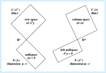
Figure: Visual representation of the four fundamental subspaces and their relationships. [1]

Guided Problems

These problems test your conceptual understanding of the Four Fundamental Subspaces, Rank, and Solvability. They minimize calculation and focus on the relationships defined by the Fundamental Theorem of Linear Algebra.

Problem 1: Rank-One Matrices and the Four Fundamental Subspaces

Let $u$ be a column vector in $\mathbb{R}^m$ and $v$ be a column vector in $\mathbb{R}^n$. Neither vector is the zero vector.

We form the $m \times n$ matrix $A$ by the outer product:

$A = uv^T$

1. Find the rank of $A$.

2. Find a basis and dimension for each of the four fundamental subspaces:

   • Column Space $C(A)$
   • Row Space $C(A^T)$
   • Nullspace $N(A)$
   • Left Nullspace $N(A^T)$

3. Describe the geometric condition for a vector $x$ to be in the nullspace.

💡 Solution

Hints:

• Rank: Write out the matrix multiplication $A = u [v_1 \dots v_n]$. Notice that every column of $A$ is a scalar multiple of the vector $u$. How many linearly independent columns does $A$ have?
• Column Space: Since every column is a multiple of $u$, what single vector spans the entire column space?
• Row Space: Recall that $\text{rank}(A^T) = \text{rank}(A)$. Alternatively, observe that every row is a multiple of $v^T$.
• Nullspace: Use the Rank-Nullity Theorem: $\dim(N(A)) = n - r$. To find the condition, write out $Ax = (uv^T)x$ and use associativity to group $(v^T x)$. For $Ax$ to be zero, what must be the value of the scalar $(v^T x)$?
• Left Nullspace: Use the Fundamental Theorem: $\dim(N(A^T)) = m - r$.

Solution:

1. Rank: $\text{rank}(A) = 1$

   • Since $u$ and $v$ are non-zero, $A$ has at least one non-zero entry. All columns are multiples of $u$, so there is only 1 independent column.

2. Four Fundamental Subspaces:

   Column Space $C(A)$:

   • Dimension: $1$
   • Basis: $\{ u \}$

   Row Space $C(A^T)$:

   • Dimension: $1$
   • Basis: $\{ v \}$

   Nullspace $N(A)$:

   • Dimension: $n - 1$
   • Basis: Any $n-1$ linearly independent vectors orthogonal to $v$
   • The nullspace is an $(n-1)$-dimensional hyperplane

   Left Nullspace $N(A^T)$:

   • Dimension: $m - 1$
   • Basis: Any $m-1$ linearly independent vectors orthogonal to $u$
   • The left nullspace is an $(m-1)$-dimensional hyperplane

3. Geometric Condition:

   • A vector $x \in \mathbb{R}^n$ is in the nullspace if and only if $x$ is orthogonal to $v$.
   • Proof: $Ax = u(v^T x)$. Since $u \neq 0$, we have $Ax = 0$ if and only if $v^T x = 0$.
   • This means $N(A) = \{ x \in \mathbb{R}^n : v^T x = 0 \}$, which is a hyperplane perpendicular to $v$.

---

Problem 2: Nullspace Preservation and the Gram Matrix

Let $A$ be a real $m \times n$ matrix. We construct the square, symmetric matrix $G = A^T A$.

1. Nullspace Equality: Show that the nullspace of $A$ is exactly the same as the nullspace of $A^T A$. (i.e., prove $N(A) = N(A^T A)$)

2. Rank Relationship: Using the result from Part 1 and the Rank-Nullity Theorem, determine the relationship between $\text{rank}(A)$ and $\text{rank}(A^T A)$.

3. Invertibility Condition: Based on Part 2, if $A$ is a tall matrix ($m > n$) with linearly independent columns, is $A^T A$ invertible? Explain your reasoning.

💡 Solution

Hints:

• Part 1: To show two sets are equal, prove both directions: (1) $N(A) \subseteq N(A^T A)$ and (2) $N(A^T A) \subseteq N(A)$. For the second direction, if $(A^T A)x = 0$, multiply both sides by $x^T$ and use the fact that $\|Ax\|^2 = (Ax)^T(Ax)$.
• Part 2: Use the Rank-Nullity Theorem: $\text{rank}(M) + \dim(N(M)) = \text{number of columns}$. Since $A$ and $A^T A$ have the same nullspace dimension and the same number of columns, what can you conclude?
• Part 3: For invertibility, check if $\text{rank}(A^T A) = n$ (full rank for a square $n \times n$ matrix). What does "linearly independent columns" tell you about $\text{rank}(A)$?

Solution:

Part 1: $N(A) = N(A^T A)$

We need to show both directions:

(1) $N(A) \subseteq N(A^T A)$:

• Let $x \in N(A)$, so $Ax = 0$.
• Then $(A^T A)x = A^T(Ax) = A^T(0) = 0$.
• Therefore $x \in N(A^T A)$.

(2) $N(A^T A) \subseteq N(A)$:

• Let $x \in N(A^T A)$, so $(A^T A)x = 0$.
• Multiply both sides by $x^T$: $x^T(A^T A)x = 0$ $(Ax)^T(Ax) = 0$ $\|Ax\|^2 = 0$
• Therefore $Ax = 0$, which means $x \in N(A)$.

Since both inclusions hold, $N(A) = N(A^T A)$.

Part 2: Rank Relationship

From Part 1, we know $N(A) = N(A^T A)$, so: $\dim(N(A)) = \dim(N(A^T A))$

Both $A$ and $A^T A$ have $n$ columns. By the Rank-Nullity Theorem:

• For $A$: $\text{rank}(A) + \dim(N(A)) = n$
• For $A^T A$: $\text{rank}(A^T A) + \dim(N(A^T A)) = n$

Since the nullspace dimensions are equal: $\boxed{\text{rank}(A^T A) = \text{rank}(A)}$

Part 3: Invertibility of $A^T A$

If $A$ is an $m \times n$ tall matrix ($m > n$) with linearly independent columns:

• "Linearly independent columns" means $\text{rank}(A) = n$ (full column rank)
• From Part 2: $\text{rank}(A^T A) = \text{rank}(A) = n$
• $A^T A$ is an $n \times n$ square matrix with rank $n$

Therefore, $A^T A$ is invertible.

Key Insight: This is why the normal equations $(A^T A)\beta = A^T b$ in linear regression have a unique solution when the columns of the design matrix $A$ are linearly independent (no perfect multicollinearity).

---

References

1. MIT OpenCourseWare - 18.06SC Linear Algebra - The Four Fundamental Subspaces
2. Strang, Gilbert - Introduction to Linear Algebra (Chapter 2)