Matrix Inverse and Invertibility

• The Central Question: Can We Undo a Transformation?
• Definition and Intuition
  • Pseudo-inverse
• Conditions for Invertibility
• Invertibility and the Four Fundamental Subspaces
  • When A is Invertible
  • When A is Singular (Not Invertible)
  • Non-Square Matrices: Structural Constraints
• Computing the Inverse
  • Method 1: Gauss-Jordan Elimination
  • Method 2: The 2×2 Formula
  • Method 3: The Adjugate Formula (General Case)
  • Method 4: LU Decomposition
• Properties of the Inverse
• The Determinant Test
• Applications in Data Science and Machine Learning
  • 1. Linear Regression (Ordinary Least Squares)
  • 2. Ridge Regression (Regularization)
  • 3. Solving Linear Systems
• Near-Singularity and Condition Number
• Guided Problems
  • Problem 1: When Does Adding a Row Make a Matrix Invertible?
  • Problem 2: Symmetric Matrix and Diagonal Perturbation
  • Problem 3: Linear Dependence and Gram Matrix
  • Problem 4: True or False — Invertibility Concepts
• Summary
• References

---

The Central Question: Can We Undo a Transformation?

Consider a linear transformation that maps vectors from $\mathbb{R}^n$ to $\mathbb{R}^m$. We encode this transformation as a matrix $A$, and applying it to a vector $x$ gives us $Ax = b$. The fundamental question of invertibility is this: given the output $b$, can we uniquely recover the input $x$?

If the answer is "yes" for every possible $b$, then the transformation preserves all information and can be undone. The matrix that undoes this transformation is called the inverse, denoted $A^{-1}$.

---

Definition and Intuition

Definition: Invertible Matrix

A square matrix $A$ (of size $n \times n$) is invertible (also called non-singular or non-degenerate) if there exists a matrix $A^{-1}$ such that:

$AA^{-1} = A^{-1}A = I$

where $I$ is the $n \times n$ identity matrix.

The inverse matrix $A^{-1}$, when it exists, is unique. Here's why: suppose both $B$ and $C$ are inverses of $A$. Then:

$B = BI = B(AC) = (BA)C = IC = C$

Geometric Intuition: Think of $A$ as a machine that transforms vectors. The inverse $A^{-1}$ is the machine that runs the transformation backwards. If $A$ stretches space by a factor of 2, then $A^{-1}$ compresses it by a factor of 2. If $A$ rotates space by 30°, then $A^{-1}$ rotates it by −30°.

Pseudo-inverse

Only square matrices can be invertible in the classical sense. A tall matrix ($m > n$) squeezes $\mathbb{R}^n$ into a subspace of $\mathbb{R}^m$—you can't get back to the full $\mathbb{R}^n$. A wide matrix ($m < n$) collapses some directions—multiple inputs map to the same output, so you can't uniquely recover the input. For non-square matrices, we use the pseudo-inverse (Moore-Penrose inverse), which gives the "best" answer in a least-squares sense.

Example: Tall Matrix ($3 \times 2$) — Not onto, can't reach all outputs

$A = \begin{bmatrix} 1 & 0 \\ 0 & 1 \\ 0 & 0 \end{bmatrix}$

This matrix takes 2D vectors and embeds them into 3D: $\begin{bmatrix} x \\ y \end{bmatrix} \mapsto \begin{bmatrix} x \\ y \\ 0 \end{bmatrix}$

The output is always in the $xy$-plane of $\mathbb{R}^3$. If someone gives you $\mathbf{b} = \begin{bmatrix} 1 \\ 2 \\ 5 \end{bmatrix}$, there's no $\mathbf{x} \in \mathbb{R}^2$ such that $A\mathbf{x} = \mathbf{b}$—you simply can't reach vectors with non-zero $z$-component. No inverse can exist because the transformation isn't onto.

Example: Wide Matrix ($2 \times 3$) — Not one-to-one, multiple inputs give same output

$B = \begin{bmatrix} 1 & 0 & 1 \\ 0 & 1 & 1 \end{bmatrix}$

This matrix projects 3D vectors down to 2D. Consider these two different inputs:

$B\begin{bmatrix} 1 \\ 1 \\ 0 \end{bmatrix} = \begin{bmatrix} 1 \\ 1 \end{bmatrix}, \quad B\begin{bmatrix} 0 \\ 0 \\ 1 \end{bmatrix} = \begin{bmatrix} 1 \\ 1 \end{bmatrix}$

Both inputs map to $\begin{bmatrix} 1 \\ 1 \end{bmatrix}$! In fact, $\begin{bmatrix} 1 \\ 1 \\ 0 \end{bmatrix}$ and $\begin{bmatrix} 0 \\ 0 \\ 1 \end{bmatrix}$ differ by $\begin{bmatrix} 1 \\ 1 \\ -1 \end{bmatrix}$, which is in the nullspace. Given an output, you can't uniquely recover the input—the transformation isn't one-to-one. No inverse can exist.

Example: Fitting a Line to Noisy Data

Suppose we have 4 data points and want to fit a line $y = mx + b$. This gives us 4 equations in 2 unknowns—an overdetermined system that generally has no exact solution. The pseudo-inverse finds the line that minimizes the sum of squared errors (residuals).

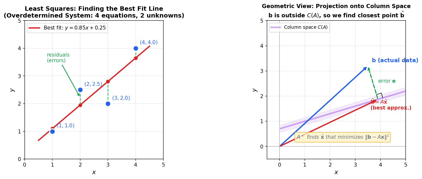
The left panel shows the data points (blue), the best-fit line (red), and the residuals (green dashed). The right panel shows the geometric interpretation: the target vector $\mathbf{b}$ lies outside the column space of $A$, so we project onto the closest point $\hat{\mathbf{b}} = A\hat{\mathbf{x}}$. The pseudo-inverse formula $\hat{\mathbf{x}} = (A^TA)^{-1}A^T\mathbf{b}$ computes this projection directly.

---

Conditions for Invertibility

For a square $n \times n$ matrix $A$, the following conditions are all equivalent. If any one is true, they are all true. If any one is false, they are all false.

Theorem: The Invertible Matrix Theorem

For an $n \times n$ matrix $A$, the following statements are equivalent:

1. $A$ is invertible
2. $A$ has full rank: $\text{rank}(A) = n$
3. The columns of $A$ are linearly independent
4. The rows of $A$ are linearly independent
5. $\det(A) \neq 0$
6. The nullspace contains only the zero vector: $N(A) = \{\mathbf{0}\}$
7. The left nullspace contains only the zero vector: $N(A^T) = \{\mathbf{0}\}$
8. The column space is all of $\mathbb{R}^n$: $C(A) = \mathbb{R}^n$
9. The row space is all of $\mathbb{R}^n$: $C(A^T) = \mathbb{R}^n$
10. The equation $Ax = b$ has a unique solution for every $b \in \mathbb{R}^n$
11. The equation $Ax = 0$ has only the trivial solution $x = 0$
12. $A$ can be row-reduced to the identity matrix $I$
13. $A$ is a product of elementary matrices
14. All eigenvalues of $A$ are non-zero

Why?

• Rank = n means all columns are independent (no redundancy), so they span all of $\mathbb{R}^n$
• If columns span $\mathbb{R}^n$, every $b$ is reachable, so $Ax = b$ always has a solution
• If columns are independent, $Ax = 0$ has only $x = 0$, so $N(A) = \{0\}$, meaning solutions are unique
• If we can reach every $b$ with a unique $x$, the transformation is one-to-one and onto—it's invertible

---

Invertibility and the Four Fundamental Subspaces

The four fundamental subspaces tell the complete story of when and why a matrix is invertible.

When $A$ is Invertible

For an invertible $n \times n$ matrix $A$:

Subspace	Dimension	Description
Column Space $C(A)$	$n$	$= \mathbb{R}^n$ (reaches everywhere)
Row Space $C(A^T)$	$n$	$= \mathbb{R}^n$ (uses all input directions)
Nullspace $N(A)$	$0$	$= \{\mathbf{0}\}$ (no information lost)
Left Nullspace $N(A^T)$	$0$	$= \{\mathbf{0}\}$ (no constraints on solvability)

An invertible matrix "preserves information" completely. No dimensions are collapsed (nullspace is trivial), and every output is reachable (column space is full). The transformation is a perfect bijection between $\mathbb{R}^n$ and $\mathbb{R}^n$.

When $A$ is Singular (Not Invertible)

When a square matrix is singular (not invertible), something has gone wrong:

Subspace	What Happens	Consequence
Nullspace $N(A)$	Contains non-zero vectors	Multiple inputs give same output
Left Nullspace $N(A^T)$	Contains non-zero vectors	Some $b$ have no solution
Column Space $C(A)$	Smaller than $\mathbb{R}^n$	Can't reach all outputs
Row Space $C(A^T)$	Smaller than $\mathbb{R}^n$	Some input directions ignored

Example: Consider the matrix $A = \begin{bmatrix} 1 & 2 \\ 2 & 4 \end{bmatrix}$

• Column 2 = 2 × Column 1, so the columns are dependent
• $\text{rank}(A) = 1 < 2$
• Nullspace: $N(A) = \text{span}\left\{\begin{bmatrix} -2 \\ 1 \end{bmatrix}\right\}$ (a line)
• Column space: $C(A) = \text{span}\left\{\begin{bmatrix} 1 \\ 2 \end{bmatrix}\right\}$ (a line, not all of $\mathbb{R}^2$)

This matrix collapses the line $\begin{bmatrix} -2 \\ 1 \end{bmatrix}t$ to zero. It's not one-to-one (multiple inputs give the same output), and it's not onto (can't reach most of $\mathbb{R}^2$).

Non-Square Matrices: Structural Constraints

For an $n \times m$ matrix $A$ (maps $\mathbb{R}^m \to \mathbb{R}^n$), the shape alone determines certain limitations:

Shape	Rank Bound	Column Space	Nullspace
Tall ($n > m$)	$\text{rank}(A) \leq m < n$	$C(A) \subsetneq \mathbb{R}^n$ (never full)	Can be $\{\mathbf{0}\}$ if full column rank
Fat ($n < m$)	$\text{rank}(A) \leq n < m$	Can equal $\mathbb{R}^n$ if full row rank	$\dim N(A) \geq m - n > 0$ (always non-trivial)

Tall matrices have more equations than unknowns. The column space lives in $\mathbb{R}^n$ but has dimension at most $m < n$, so it cannot fill $\mathbb{R}^n$. Most target vectors $\mathbf{b}$ have no solution—the system is overdetermined.

Fat matrices have more unknowns than equations. The nullspace has dimension at least $m - n > 0$, so non-trivial vectors always get mapped to zero. Multiple inputs produce the same output—the system is underdetermined.

Only square matrices can potentially be both one-to-one (trivial nullspace) and onto (full column space) simultaneously.

---

Computing the Inverse

There are several methods to compute the inverse of a matrix. Each has its place depending on the context.

Method 1: Gauss-Jordan Elimination

The most general method works for any invertible matrix. The idea: apply the same row operations that reduce $A$ to $I$ to the identity matrix $I$; the result is $A^{-1}$.

Procedure: Form the augmented matrix $[A \mid I]$ and row-reduce to $[I \mid A^{-1}]$.

Example: Find the inverse of $A = \begin{bmatrix} 2 & 1 \\ 5 & 3 \end{bmatrix}$

$\left[\begin{array}{cc|cc} 2 & 1 & 1 & 0 \\ 5 & 3 & 0 & 1 \end{array}\right]$

Step 1: $R_1 \leftarrow \frac{1}{2}R_1$: $\left[\begin{array}{cc|cc} 1 & \frac{1}{2} & \frac{1}{2} & 0 \\ 5 & 3 & 0 & 1 \end{array}\right]$

Step 2: $R_2 \leftarrow R_2 - 5R_1$: $\left[\begin{array}{cc|cc} 1 & \frac{1}{2} & \frac{1}{2} & 0 \\ 0 & \frac{1}{2} & -\frac{5}{2} & 1 \end{array}\right]$

Step 3: $R_2 \leftarrow 2R_2$: $\left[\begin{array}{cc|cc} 1 & \frac{1}{2} & \frac{1}{2} & 0 \\ 0 & 1 & -5 & 2 \end{array}\right]$

Step 4: $R_1 \leftarrow R_1 - \frac{1}{2}R_2$: $\left[\begin{array}{cc|cc} 1 & 0 & 3 & -1 \\ 0 & 1 & -5 & 2 \end{array}\right]$

Therefore: $A^{-1} = \begin{bmatrix} 3 & -1 \\ -5 & 2 \end{bmatrix}$

Verification: $AA^{-1} = \begin{bmatrix} 2 & 1 \\ 5 & 3 \end{bmatrix}\begin{bmatrix} 3 & -1 \\ -5 & 2 \end{bmatrix} = \begin{bmatrix} 1 & 0 \\ 0 & 1 \end{bmatrix}$ ✓

Method 2: The 2×2 Formula

For $2 \times 2$ matrices, there's a closed-form formula:

Formula: 2×2 Inverse

If $A = \begin{bmatrix} a & b \\ c & d \end{bmatrix}$ and $\det(A) = ad - bc \neq 0$, then:

$A^{-1} = \frac{1}{ad - bc}\begin{bmatrix} d & -b \\ -c & a \end{bmatrix}$

Method 3: The Adjugate Formula (General Case)

For any $n \times n$ matrix:

$A^{-1} = \frac{1}{\det(A)} \text{adj}(A)$

where $\text{adj}(A)$ is the adjugate matrix (transpose of the matrix of cofactors). This formula is theoretically elegant but computationally expensive for large matrices.

Method 4: LU Decomposition

For numerical computation, factoring $A = LU$ (lower × upper triangular) allows efficient solving of $Ax = b$ without explicitly computing $A^{-1}$. This is the standard approach in numerical libraries.

---

Properties of the Inverse

Theorem: Properties of Matrix Inverse

If $A$ and $B$ are invertible $n \times n$ matrices, then:

1. Inverse of inverse: $(A^{-1})^{-1} = A$
2. Inverse of product: $(AB)^{-1} = B^{-1}A^{-1}$ (note the reversed order!)
3. Inverse of transpose: $(A^T)^{-1} = (A^{-1})^T$
4. Inverse of scalar multiple: $(cA)^{-1} = \frac{1}{c}A^{-1}$ for $c \neq 0$
5. Determinant of inverse: $\det(A^{-1}) = \frac{1}{\det(A)}$

Why does the product reverse? Think of putting on socks and shoes: if $A$ = "put on socks" and $B$ = "put on shoes", then $(AB)^{-1}$ must first undo $B$ (take off shoes), then undo $A$ (take off socks). Hence $(AB)^{-1} = B^{-1}A^{-1}$.

---

The Determinant Test

The determinant provides a single-number test for invertibility:

The Determinant Rule

A square matrix $A$ is invertible if and only if $\det(A) \neq 0$.

The determinant measures the signed volume scaling factor of the transformation. If $\det(A) = 0$, the transformation collapses some dimension—the volume becomes zero. A collapsed dimension can't be recovered, so the matrix isn't invertible.

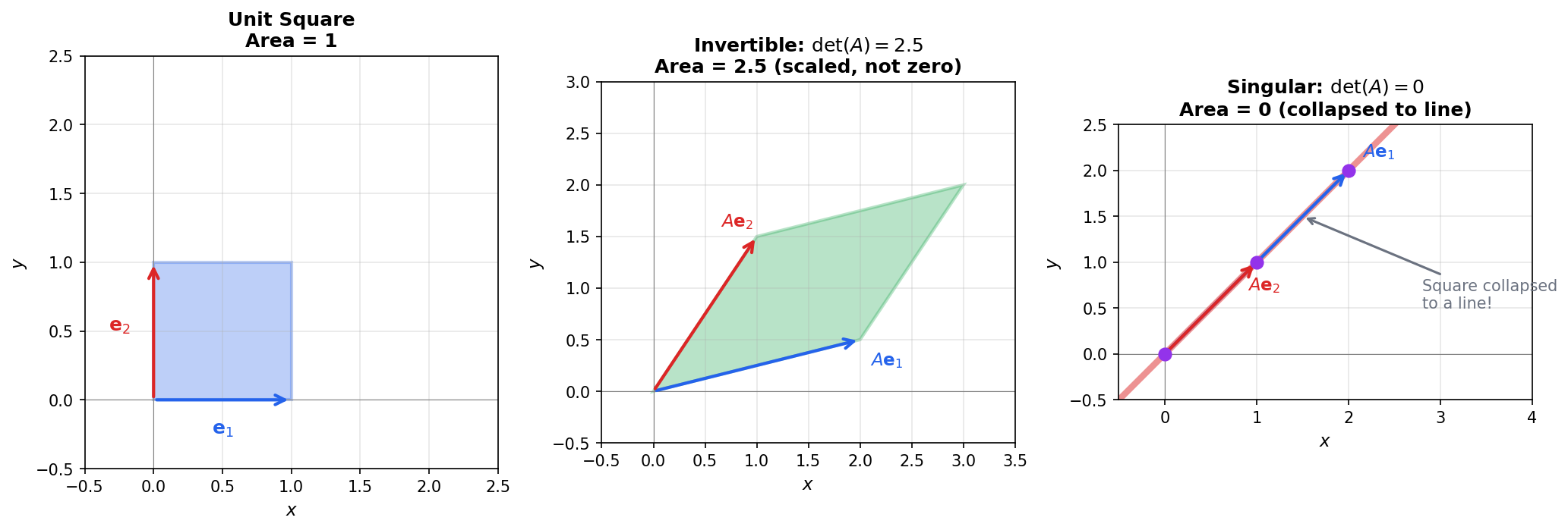
The unit square (left) transforms to a parallelogram with area $= |\det(A)|$. An invertible matrix (middle) scales area but keeps it non-zero. A singular matrix (right) collapses the square to a line—area becomes zero, and the original shape cannot be recovered.

Examples:

• $\det\begin{bmatrix} 2 & 1 \\ 5 & 3 \end{bmatrix} = 6 - 5 = 1 \neq 0$ → Invertible
• $\det\begin{bmatrix} 1 & 2 \\ 2 & 4 \end{bmatrix} = 4 - 4 = 0$ → Singular

---

Applications in Data Science and Machine Learning

1. Linear Regression (Ordinary Least Squares)

The normal equations for OLS are:

$(X^T X)\beta = X^T y$

where $X$ is the $m \times n$ design matrix ($m$ samples, $n$ features), $y \in \mathbb{R}^m$ is the target vector, and $\beta \in \mathbb{R}^n$ are the coefficients we want to find.

The Gram Matrix $G = X^T X$ must be invertible to get a unique solution:

$\beta = (X^T X)^{-1} X^T y$

When is $X^TX$ invertible?

• The columns of $X$ must be linearly independent
• There must be no perfect multicollinearity (no feature is a linear combination of others)
• You need at least as many samples as features ($m \geq n$)

What goes wrong when $X^TX$ is singular?

When $X^TX$ is singular, $N(X^TX) = N(X) \neq \{\mathbf{0}\}$, meaning some non-zero vector $\mathbf{v}$ satisfies $X\mathbf{v} = \mathbf{0}$.

Why $N(X^TX) = N(X)$?

• $N(X) \subseteq N(X^TX)$: If $X\mathbf{v} = \mathbf{0}$, then $X^TX\mathbf{v} = X^T\mathbf{0} = \mathbf{0}$.
• $N(X^TX) \subseteq N(X)$: If $X^TX\mathbf{v} = \mathbf{0}$, multiply both sides by $\mathbf{v}^T$: $\mathbf{v}^TX^TX\mathbf{v} = \|X\mathbf{v}\|^2 = 0$. A vector with zero norm must be $\mathbf{0}$, so $X\mathbf{v} = \mathbf{0}$.

1. Non-unique coefficients: If $\beta^*$ is a solution, then $\beta^* + t\mathbf{v}$ is also a solution for any scalar $t$, because $X(\beta^* + t\mathbf{v}) = X\beta^* + tX\mathbf{v} = X\beta^*$. The solution space is an affine subspace, not a single point.

2. Interpretability breaks down: Suppose features $x_2 = 2x_1$ (perfect multicollinearity). Then $\beta_1 = 5, \beta_2 = 0$ and $\beta_1 = 1, \beta_2 = 2$ produce identical predictions. You cannot attribute effect to individual features.

3. Numerical instability: Even if $X^TX$ is technically invertible but nearly singular (high condition number), floating-point errors get amplified. A condition number of $10^8$ with double precision ($\sim 16$ digits) leaves only $\sim 8$ reliable digits in $\beta$.

2. Ridge Regression (Regularization)

When $X^TX$ is singular or nearly singular, we add a regularization term:

$(X^T X + \lambda I)\beta = X^T y$

Why does this help?

Adding $\lambda I$ eliminates the nullspace. Suppose $\mathbf{v} \in N(X^TX + \lambda I)$, meaning $(X^TX + \lambda I)\mathbf{v} = \mathbf{0}$. Then:

$X^TX\mathbf{v} = -\lambda\mathbf{v}$

Taking the inner product with $\mathbf{v}$:

$\mathbf{v}^TX^TX\mathbf{v} = -\lambda\mathbf{v}^T\mathbf{v}$ $\|X\mathbf{v}\|^2 = -\lambda\|\mathbf{v}\|^2$

The left side is $\geq 0$. The right side is $\leq 0$ when $\lambda > 0$ (and strictly negative if $\mathbf{v} \neq \mathbf{0}$). The only solution is $\mathbf{v} = \mathbf{0}$. Therefore $N(X^TX + \lambda I) = \{\mathbf{0}\}$, so the matrix is invertible.

Eigenvalue perspective

The "flat direction" $\mathbf{v}$ is an eigenvector of $X^TX$ with a small eigenvalue $\lambda_i \approx 0$. Eigenvalues measure curvature: $X^TX\mathbf{v} = \lambda_i\mathbf{v}$ means moving along $\mathbf{v}$ changes the loss by only $\lambda_i\|\mathbf{v}\|^2$—nearly zero if $\lambda_i \approx 0$.

If $X^TX$ has eigenvalues $\lambda_1, \lambda_2, \ldots, \lambda_n$, then $X^TX + \lambda I$ has eigenvalues $\lambda_1 + \lambda, \lambda_2 + \lambda, \ldots, \lambda_n + \lambda$. The flat directions (small $\lambda_i$) become steep (now $\lambda_i + \lambda$). If some $\lambda_i = 0$ (singular), adding $\lambda > 0$ shifts all eigenvalues positive, making the matrix invertible.

Trade-off: Regularization introduces bias (the solution is no longer exactly optimal for the training data) but reduces variance (the solution is more stable—small changes in data don't cause large swings in $\beta$).

When $X^TX$ is nearly singular, there exists a direction $\mathbf{v}$ where $X^TX\mathbf{v} \approx \mathbf{0}$. The solution can "slide" along $\mathbf{v}$ with almost no change in the loss $\|X\beta - y\|^2$. Small noise in $y$ can push $\beta$ far along this flat direction.

Adding $\lambda I$ penalizes movement in all directions equally. Now sliding along $\mathbf{v}$ costs $\lambda\|\mathbf{v}\|^2$, anchoring the solution near the origin. The flatter the original direction, the more regularization helps.

3. Solving Linear Systems

Whenever we need to solve $Ax = b$:

• Invertible $A$: Unique solution $x = A^{-1}b$
• Singular $A$: Either no solution or infinitely many solutions

In practice, we rarely compute $A^{-1}$ explicitly. Instead, we use matrix factorizations (LU, QR, Cholesky) that solve $Ax = b$ more efficiently and stably.

---

Near-Singularity and Condition Number

In numerical computing, a matrix can be "technically invertible" but still cause problems. This happens when the matrix is ill-conditioned—close to being singular.

Definition: Condition Number

The condition number of a matrix $A$ is:

$\kappa(A) = \|A\| \cdot \|A^{-1}\|$

or equivalently (for the 2-norm):

$\kappa(A) = \frac{\sigma_{\max}}{\sigma_{\min}}$

where $\sigma_{\max}$ and $\sigma_{\min}$ are the largest and smallest singular values of $A$.

Interpretation:

• $\kappa(A) \approx 1$: Well-conditioned; small errors in $b$ cause small errors in $x$
• $\kappa(A) \gg 1$: Ill-conditioned; small errors in $b$ can cause large errors in $x$
• $\kappa(A) = \infty$: Singular matrix

Example: Calculating $\kappa$

For $A = \begin{bmatrix} 4 & 0 \\ 0 & 0.01 \end{bmatrix}$ (diagonal matrix):

• Singular values = absolute values of diagonal entries: $\sigma_{\max} = 4$, $\sigma_{\min} = 0.01$
• $\kappa(A) = \frac{4}{0.01} = 400$

For $A = \begin{bmatrix} 1 & 1 \\ 1 & 1.001 \end{bmatrix}$ (nearly singular):

• Compute $A^TA = \begin{bmatrix} 2 & 2.001 \\ 2.001 & 2.002001 \end{bmatrix}$
• Eigenvalues of $A^TA$: $\lambda_1 \approx 4.002$, $\lambda_2 \approx 0.000001$
• Singular values: $\sigma_{\max} = \sqrt{4.002} \approx 2$, $\sigma_{\min} = \sqrt{0.000001} = 0.001$
• $\kappa(A) = \frac{2}{0.001} = 2000$

The tiny $\sigma_{\min}$ signals a nearly flat direction—small changes in $\mathbf{b}$ along this direction get amplified by $1/\sigma_{\min} = 1000$.

Rule of thumb: If $\kappa(A) = 10^k$ and you're working with $d$ digits of precision, expect to lose about $k$ digits of accuracy when solving $Ax = b$.

Practical advice:

• Check the condition number before inverting matrices
• Prefer factorization methods (LU, QR) over explicit inversion
• Use regularization for ill-conditioned problems

---

Guided Problems

Problem 1: When Does Adding a Row Make a Matrix Invertible?

Consider the $2 \times 3$ matrix:

$A = \begin{bmatrix} 1 & 2 & 3 \\ 4 & 5 & 6 \end{bmatrix}$

1. Is $A$ invertible? Explain why or why not using the shape of the matrix.

2. Suppose we add a third row to create a $3 \times 3$ matrix $B$. Can you choose a third row such that $B$ is invertible? If yes, give an example. If no, explain why.

3. Now consider removing a column from $A$ to get a $2 \times 2$ matrix $C$. Which column(s) can you remove to make $C$ invertible?

💡 Solution

Part 1: $A$ is not invertible because it's not square. A $2 \times 3$ matrix maps $\mathbb{R}^3 \to \mathbb{R}^2$. It has a non-trivial nullspace (dimension $\geq 3 - 2 = 1$), so multiple inputs map to the same output. No inverse can exist.

Part 2: We need to check if rows 1 and 2 are linearly independent first. Row 2 = Row 1 + $\begin{bmatrix} 3 & 3 & 3 \end{bmatrix}$, so they are independent.

For $B$ to be invertible, the third row must not be in the span of the first two rows.

Example: $\mathbf{r}_3 = \begin{bmatrix} 0 & 0 & 1 \end{bmatrix}$ works.

$B = \begin{bmatrix} 1 & 2 & 3 \\ 4 & 5 & 6 \\ 0 & 0 & 1 \end{bmatrix}$

Check: $\det(B) = 1(5 \cdot 1 - 6 \cdot 0) - 2(4 \cdot 1 - 6 \cdot 0) + 3(4 \cdot 0 - 5 \cdot 0) = 5 - 8 + 0 = -3 \neq 0$. ✓

Part 3: Removing column 3 gives $C = \begin{bmatrix} 1 & 2 \\ 4 & 5 \end{bmatrix}$, with $\det(C) = 5 - 8 = -3 \neq 0$. Invertible. ✓

Removing column 2 gives $C = \begin{bmatrix} 1 & 3 \\ 4 & 6 \end{bmatrix}$, with $\det(C) = 6 - 12 = -6 \neq 0$. Invertible. ✓

Removing column 1 gives $C = \begin{bmatrix} 2 & 3 \\ 5 & 6 \end{bmatrix}$, with $\det(C) = 12 - 15 = -3 \neq 0$. Invertible. ✓

All three choices work because no two columns of $A$ are parallel.

---

Problem 2: Symmetric Matrix and Diagonal Perturbation

Let $S$ be a $4 \times 4$ symmetric matrix defined as follows:

$$S = \begin{bmatrix} 1 & 1 & 0 & 0 \\ 1 & 1 & 0 & 0 \\ 0 & 0 & 2 & 0 \\ 0 & 0 & 0 & 3 \end{bmatrix}$$

1. Find the rank of $S$ and a basis for its Nullspace, $N(S)$. Is $S$ invertible?

2. Let $\lambda$ be a positive scalar (e.g., $\lambda = 0.5$). We construct a new matrix $P$ by adding $\lambda$ to the diagonal of $S$:

   $$P = S + \lambda I$$

   Find the rank of this new matrix $P$. Is $P$ invertible?

💡 Solution

Part 1: Analyzing Matrix $S$

To find the rank and nullspace, we perform Gaussian elimination to reach Row Echelon Form.

$$\begin{bmatrix} 1 & 1 & 0 & 0 \\ 1 & 1 & 0 & 0 \\ 0 & 0 & 2 & 0 \\ 0 & 0 & 0 & 3 \end{bmatrix} \xrightarrow{R_2 - R_1} \begin{bmatrix} \mathbf{1} & 1 & 0 & 0 \\ 0 & 0 & 0 & 0 \\ 0 & 0 & \mathbf{2} & 0 \\ 0 & 0 & 0 & \mathbf{3} \end{bmatrix}$$

Rearranging the zero row to the bottom:

$$U = \begin{bmatrix} \mathbf{1} & 1 & 0 & 0 \\ 0 & 0 & \mathbf{2} & 0 \\ 0 & 0 & 0 & \mathbf{3} \\ 0 & 0 & 0 & 0 \end{bmatrix}$$

• Rank: There are 3 pivots (in columns 1, 3, and 4). Therefore, $\text{rank}(S) = 3$.
• Invertibility: Since the rank (3) is less than the dimension (4), the matrix is singular (not invertible).
• Nullspace Basis: There is one free variable corresponding to column 2 ($x_2$). The equation from row 1 is: $x_1 + x_2 = 0 \implies x_1 = -x_2$. The other rows imply $x_3 = 0$ and $x_4 = 0$. Setting free variable $x_2 = 1$: $$\mathcal{B}_{null} = \left\{ \begin{bmatrix} -1 \\ 1 \\ 0 \\ 0 \end{bmatrix} \right\}$$

Part 2: Analyzing the Perturbed Matrix $P = S + \lambda I$

We add $\lambda$ (where $\lambda > 0$) to the diagonal elements of $S$.

$$P = \begin{bmatrix} 1+\lambda & 1 & 0 & 0 \\ 1 & 1+\lambda & 0 & 0 \\ 0 & 0 & 2+\lambda & 0 \\ 0 & 0 & 0 & 3+\lambda \end{bmatrix}$$

To check the rank/invertibility, we can check the determinant. Since the matrix is block diagonal, the determinant is the product of the determinants of the blocks.

Block 1 (Top-Left $2\times2$):

$$\det \left( \begin{bmatrix} 1+\lambda & 1 \\ 1 & 1+\lambda \end{bmatrix} \right) = (1+\lambda)(1+\lambda) - (1)(1)$$$$= (1 + 2\lambda + \lambda^2) - 1 = 2\lambda + \lambda^2$$

Block 2 (Bottom-Right Diagonal): The determinants are simply the diagonal entries: $(2+\lambda)$ and $(3+\lambda)$.

Total Determinant:

$$\det(P) = (2\lambda + \lambda^2) \cdot (2+\lambda) \cdot (3+\lambda)$$

Conclusion: Since $\lambda$ is positive ($\lambda > 0$), every term in that product is positive. Therefore, $\det(P) \neq 0$.

• Invertibility: The matrix $P$ is invertible.
• Rank: Since it is invertible, it must have full rank. $\text{rank}(P) = 4$.

Connection Summary: Even though the original matrix $S$ lost information (rank 3, non-invertible), adding a small scalar matrix $\lambda I$ restored the rank to 4, making the system solvable for a unique solution. This is exactly what Ridge Regression does!

---

Problem 3: Linear Dependence and Gram Matrix

Let $A$ be a $4 \times 3$ matrix defined as:

$$A = \begin{bmatrix} 1 & 2 & 3 \\ 1 & 3 & 4 \\ 1 & 4 & 5 \\ 1 & 5 & 6 \end{bmatrix}$$

1. Determine if the columns of $A$ are linearly independent. If they are dependent, find a non-zero vector $\mathbf{x}$ such that $A\mathbf{x} = \mathbf{0}$.

2. Calculate the symmetric matrix $G = A^T A$.

3. Without performing full Gaussian elimination on $G$, determine the rank of $G$ and whether $G$ is invertible. Explain your reasoning based on the result from Part 1.

💡 Solution

Part 1: Linear Independence and Nullspace

We examine the columns of $A$:

$$c_3 = c_1 + c_2$$

Since $\mathbf{c}_3$ can be written as a linear combination of $\mathbf{c}_1$ and $\mathbf{c}_2$, the columns are linearly dependent.

To find the vector $\mathbf{x}$ (which is in the Nullspace $N(A)$), we rewrite the dependency equation:

$$1\cdot\mathbf{c}_1 + 1\cdot\mathbf{c}_2 - 1\cdot\mathbf{c}_3 = \mathbf{0}$$

This gives us the coefficients for our vector $\mathbf{x}$:

$$\mathbf{x} = \begin{bmatrix} 1 \\ 1 \\ -1 \end{bmatrix}$$

Part 2: Calculating $G = A^T A$

$$G = \begin{bmatrix} 1 & 1 & 1 & 1 \\ 2 & 3 & 4 & 5 \\ 3 & 4 & 5 & 6 \end{bmatrix} \begin{bmatrix} 1 & 2 & 3 \\ 1 & 3 & 4 \\ 1 & 4 & 5 \\ 1 & 5 & 6 \end{bmatrix}$$$$G = \begin{bmatrix} 4 & 14 & 18 \\ 14 & 54 & 68 \\ 18 & 68 & 86 \end{bmatrix}$$

Part 3: Rank and Invertibility of $G$

Key Fact: $\text{rank}(A^T A) = \text{rank}(A)$ (see Vector Spaces Deep Dive for proof)

1. Rank of A: Since column 3 is dependent on columns 1 and 2 (and columns 1 and 2 are independent of each other), $\text{rank}(A) = 2$.
2. Rank of G: Therefore, $\text{rank}(G) = \text{rank}(A^T A) = \text{rank}(A) = 2$.
3. Invertibility: The matrix $G$ is a $3 \times 3$ matrix. For a $3 \times 3$ matrix to be invertible, it must have full rank (rank = 3).
   • Since $\text{rank}(G) = 2 < 3$, $G$ is not invertible (it is singular).

Mathematical Connection to Data Science

This problem illustrates Perfect Multicollinearity.

1. The Matrix $A$ (Feature Matrix): Imagine $A$ represents your data. Column 1 is a bias term, Column 2 is "Feature A", and Column 3 is "Feature B". The math shows that Feature B is exactly Feature A plus the bias. They contain redundant information.
2. The Vector $\mathbf{x}$ (Non-uniqueness): The existence of a non-zero vector $\mathbf{x}$ in the nullspace means there are infinite ways to combine the features to get the same result. The weights are not unique.
3. The Matrix $G$ (Hessian/Gram Matrix): In optimization (OLS), we must invert $G = A^T A$. Because the columns were dependent, $G$ became singular. You literally cannot calculate $(A^T A)^{-1}$, causing the algorithm to crash or output "NaN".

---

Problem 4: True or False — Invertibility Concepts

For each statement, determine if it is True or False. Justify your answer.

1. If $A$ and $B$ are both invertible $n \times n$ matrices, then $A + B$ is also invertible.

2. If $A^2$ is invertible, then $A$ is invertible.

3. If $AB = I$, then $BA = I$.

4. If $A$ is invertible and $A\mathbf{x} = A\mathbf{y}$, then $\mathbf{x} = \mathbf{y}$.

💡 Solution

1. False.

Counterexample: Let $A = I$ and $B = -I$. Both are invertible, but $A + B = I + (-I) = 0$, which is not invertible.

2. True.

If $A^2$ is invertible, then $\det(A^2) \neq 0$. Since $\det(A^2) = (\det(A))^2$, we have $(\det(A))^2 \neq 0$, which means $\det(A) \neq 0$. Therefore $A$ is invertible.

3. True (when $A$ and $B$ are square matrices of the same size).

If $AB = I$, then $B$ is a right inverse of $A$. For square matrices, a right inverse is also a left inverse.

Proof: From $AB = I$, we have $\det(A)\det(B) = 1$, so $\det(A) \neq 0$ and $\det(B) \neq 0$. Thus both $A$ and $B$ are invertible. Then $B = IB = (A^{-1}A)B = A^{-1}(AB) = A^{-1}I = A^{-1}$. So $BA = A^{-1}A = I$.

4. True.

If $A\mathbf{x} = A\mathbf{y}$, then $A(\mathbf{x} - \mathbf{y}) = \mathbf{0}$. Since $A$ is invertible, $N(A) = \{\mathbf{0}\}$, so $\mathbf{x} - \mathbf{y} = \mathbf{0}$, meaning $\mathbf{x} = \mathbf{y}$.

Alternatively: multiply both sides by $A^{-1}$: $A^{-1}A\mathbf{x} = A^{-1}A\mathbf{y}$, giving $\mathbf{x} = \mathbf{y}$.

---

Summary

Invertibility fundamentals:

• A square matrix $A$ is invertible if $AA^{-1} = A^{-1}A = I$; the inverse is unique when it exists
• Non-square matrices cannot be invertible: tall matrices aren't onto, wide matrices aren't one-to-one
• For non-square systems, the pseudo-inverse provides the least-squares best answer

Equivalent conditions (Invertible Matrix Theorem):

• Full rank ($\text{rank}(A) = n$)
• Linearly independent columns (and rows)
• Trivial nullspace: $N(A) = \{\mathbf{0}\}$
• Non-zero determinant: $\det(A) \neq 0$
• Column space spans $\mathbb{R}^n$: $C(A) = \mathbb{R}^n$

Four fundamental subspaces view:

• Invertible: all four subspaces have "perfect" dimensions (column/row space = $\mathbb{R}^n$, nullspaces = $\{\mathbf{0}\}$)
• Singular: some dimension collapses (non-trivial nullspace), some outputs unreachable (column space $\subsetneq \mathbb{R}^n$)

Computing and testing:

• Gauss-Jordan elimination: row-reduce $[A \mid I]$ to $[I \mid A^{-1}]$
• The $2 \times 2$ formula: $A^{-1} = \frac{1}{ad-bc}\begin{bmatrix} d & -b \\ -c & a \end{bmatrix}$
• Determinant test: $\det(A) = 0$ iff the transformation collapses volume to zero

Applications:

• Linear regression requires $(X^TX)^{-1}$; singular $X^TX$ means non-unique coefficients
• Ridge regression adds $\lambda I$ to eliminate the nullspace, guaranteeing invertibility
• Condition number $\kappa = \sigma_{\max}/\sigma_{\min}$ measures numerical stability; high $\kappa$ amplifies errors

---

References

1. Strang, Gilbert - Introduction to Linear Algebra (Chapters 2-3)
2. MIT OpenCourseWare - 18.06SC Linear Algebra
3. Golub, Gene H. and Van Loan, Charles F. - Matrix Computations (Chapter 2)